Before you begin
What you’ll learn
- Projections
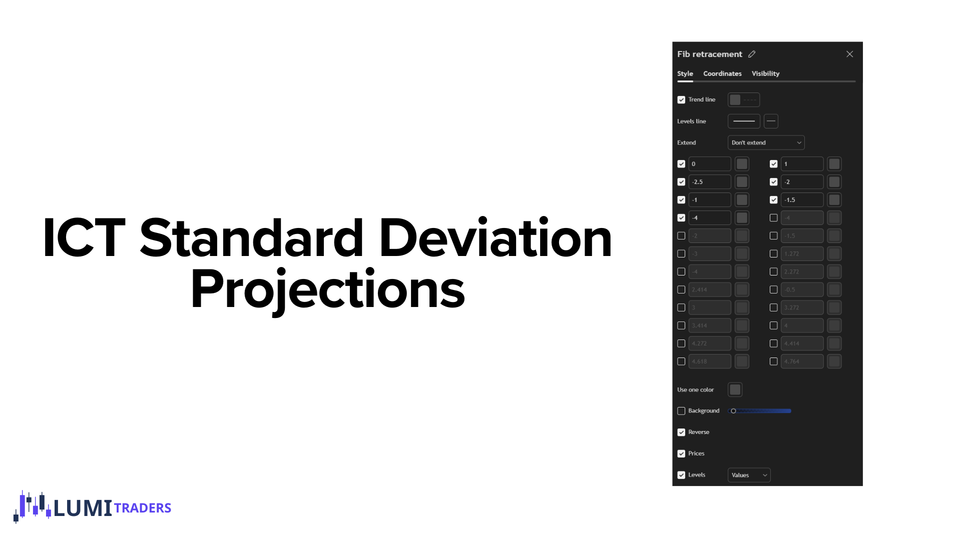
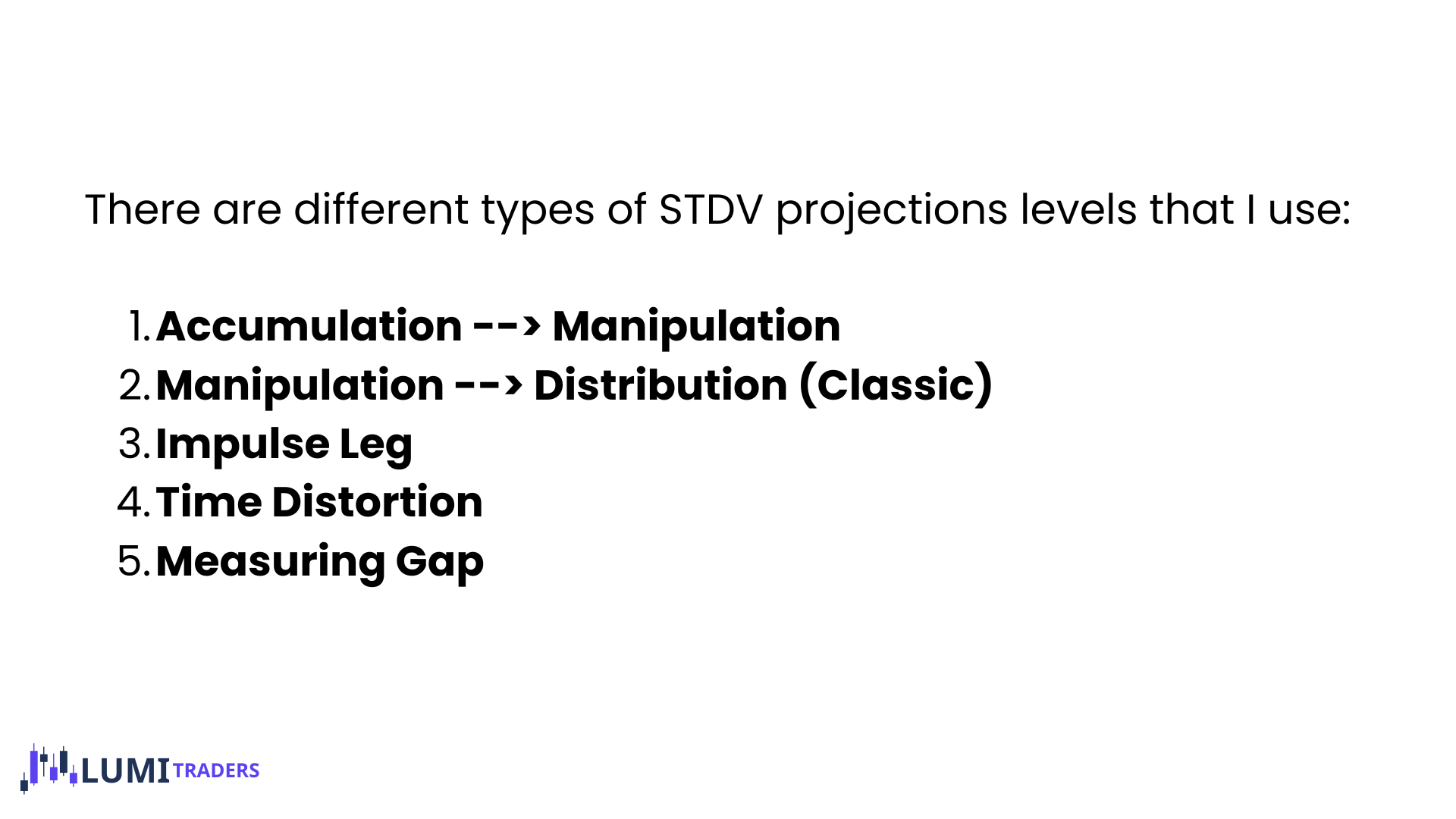
Basic explanation of Standard Deviations is a potential target of MMXM. In other words, we use STDV to anticipate a zone of reversal or retracement.
Accumulation Leg
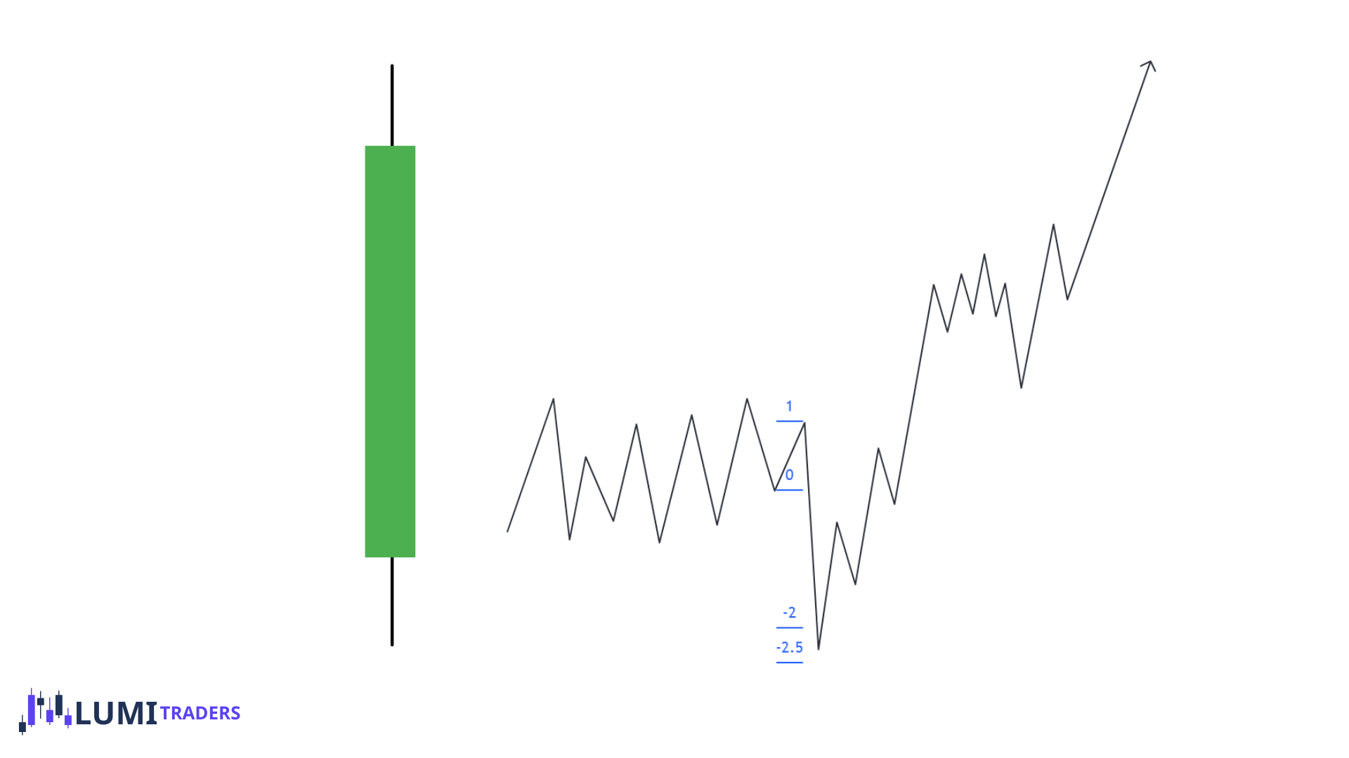
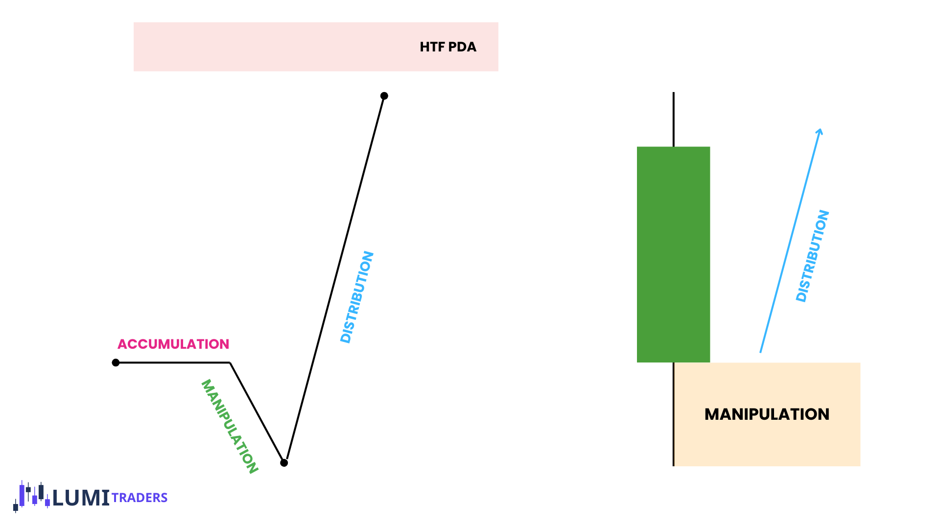
Accumulation is where "smart money," accumulate positions to set up framework for distribution phase. During this phase, price action usually range-bound, with low volatility and relatively small price movements.
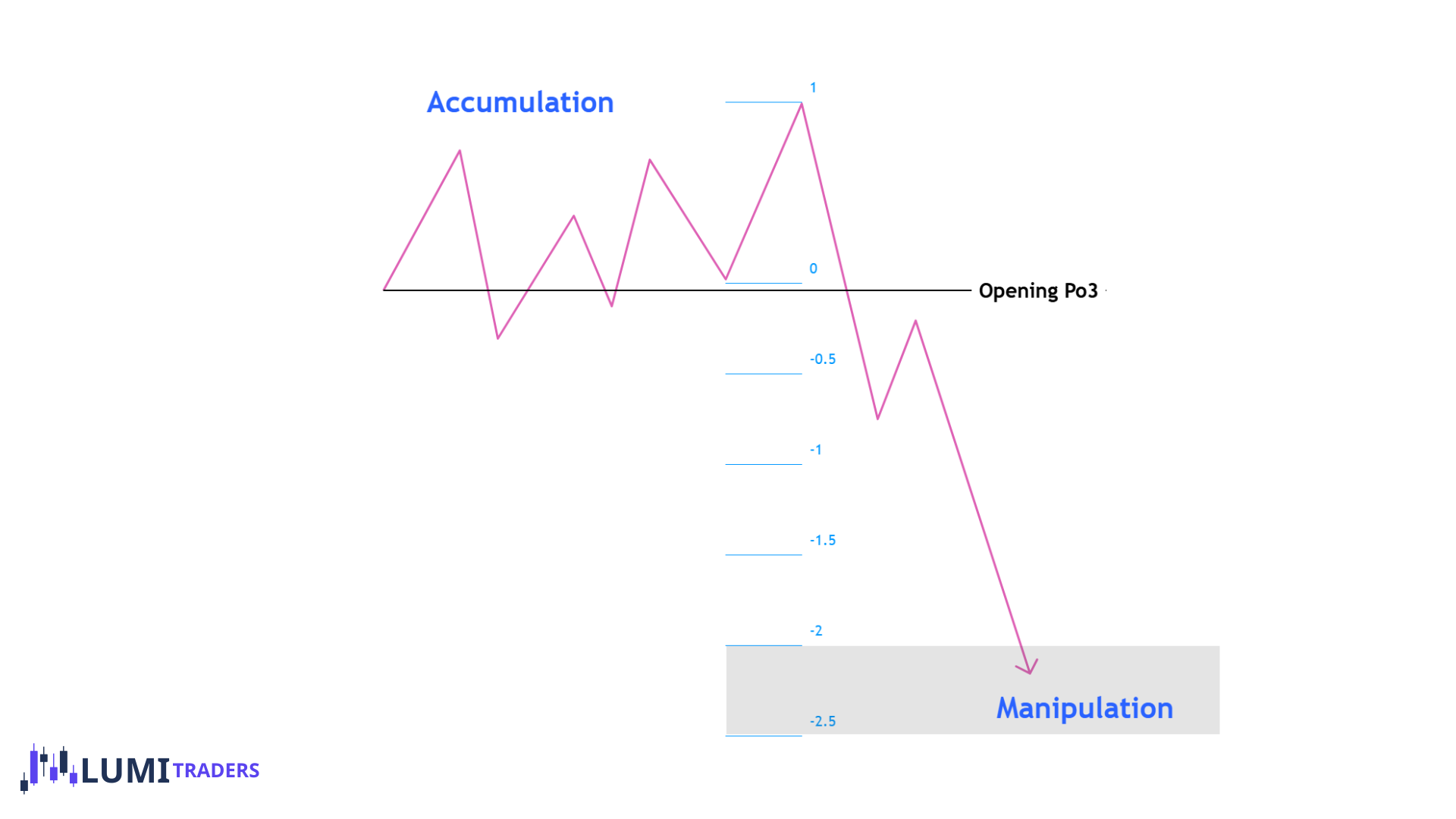
We can see accumulation (consolidation) above/below or near opening price.
In Accumulation phase, we see consolidation where a lot of liquidity is generated and then we see a fake move (manipulation) to clear all the liquidity and then SMR.
Standard Deviation: Accumulation Phase
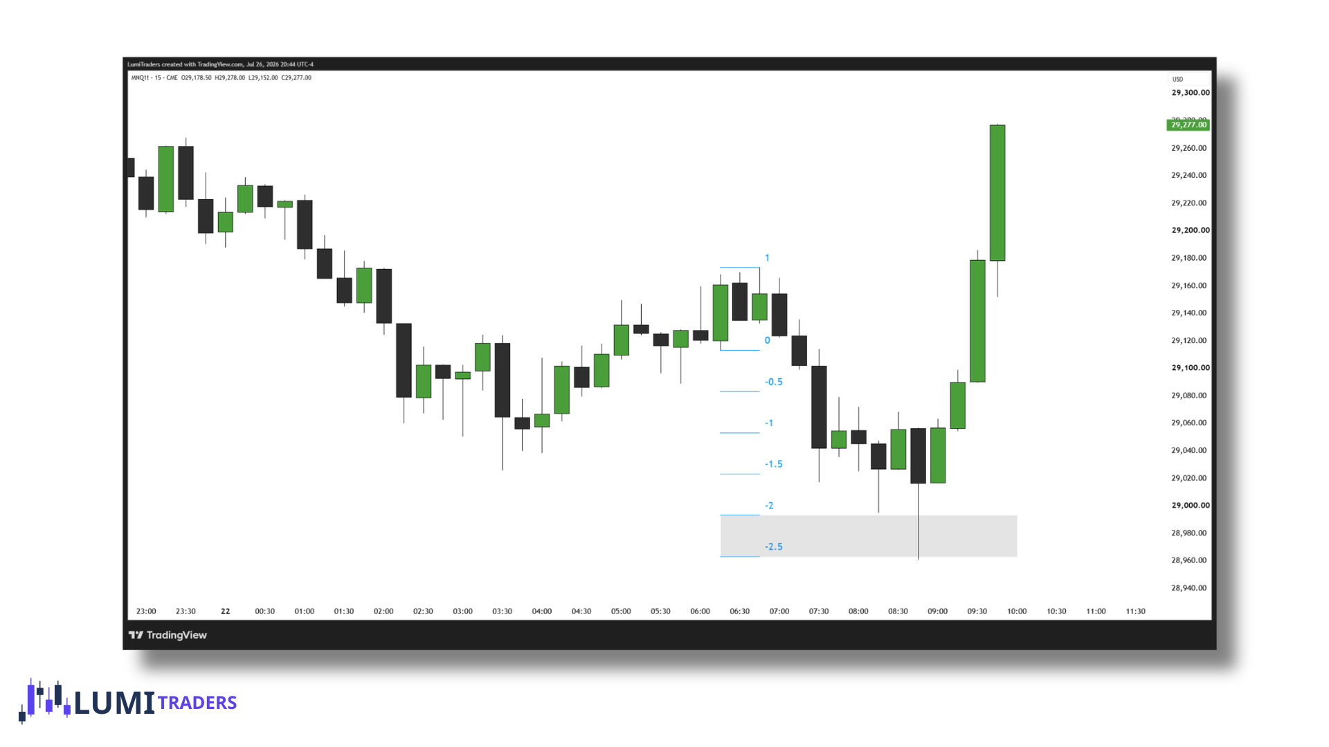
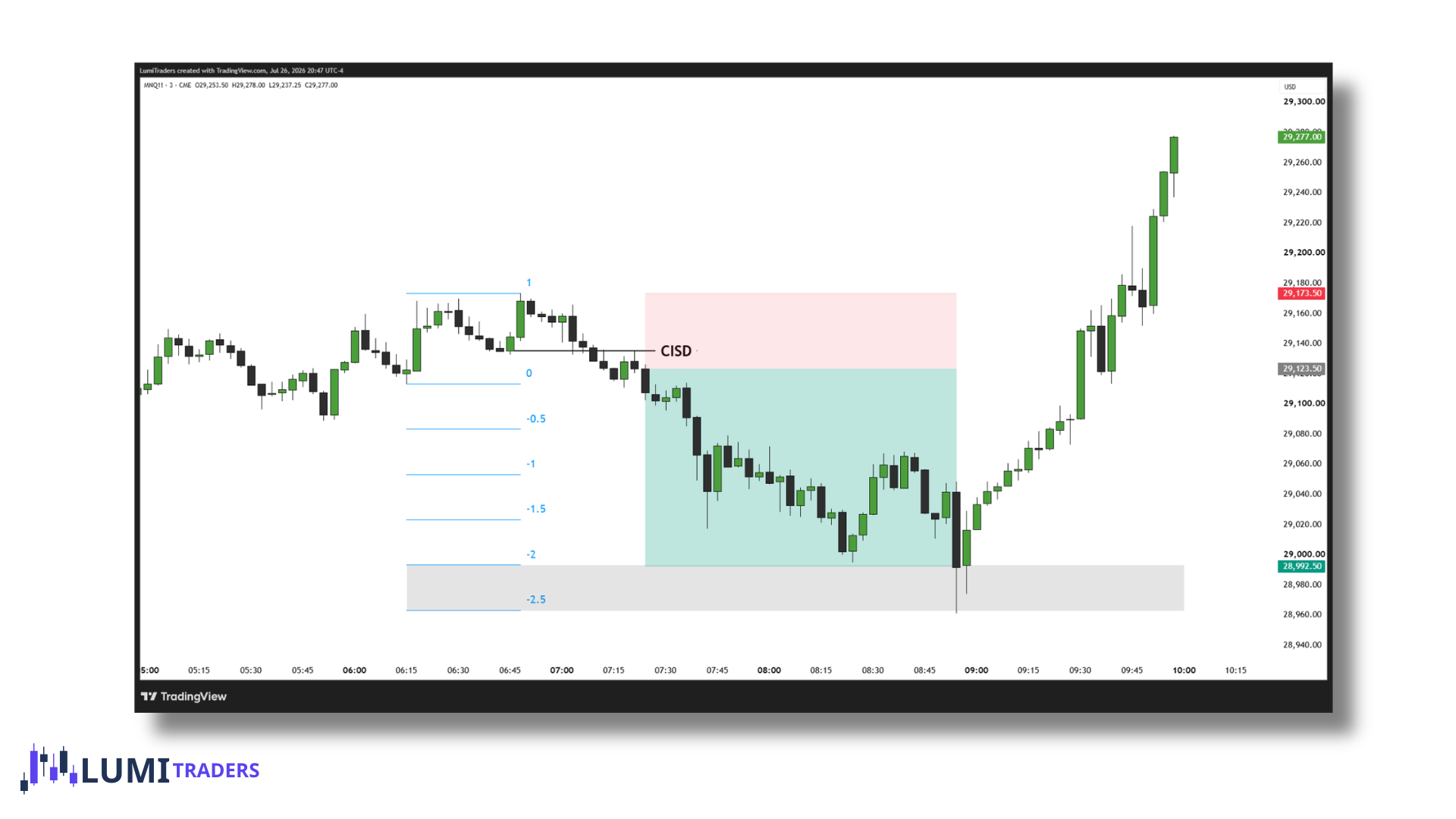
During the Accumulation, the lowest/highest obvious and visible range measured from the low/high to the high/low will project the Manipulation.
Note: 2-2.5 Standard Deviation zone is used to anticipate manipulation.
Can I trade the move from consolidation?
Yes, you can trade the move from the consolidation toward the HTF level, or target the 2 STD and 2.5 STD ranges.
What is the best entry for this setup?
The best entry is typically the change in the state of delivery (CISD) / Order Block (OB) that forms near the 50% level of the consolidation.
You may see price break above or below the consolidation and then immediately return back into the range. Most of the time, we see this quick retracement back into the range to retest the change in the state of delivery near the 50% level of the accumulation.
However, this does not mean we have to wait for price to break above or below the consolidation before looking for a retest of the OB.
The retest can happen within the consolidation itself.
Manipulation Leg
Manipulation is where smart money engineers price moves to create liquidity.
They do this by running price above or below the accumulation phase.
In other words, manipulation is where fake move occurs in the opposite direction of a key HTF PDA.
Basically, it is the wick (high/low) that is developing.
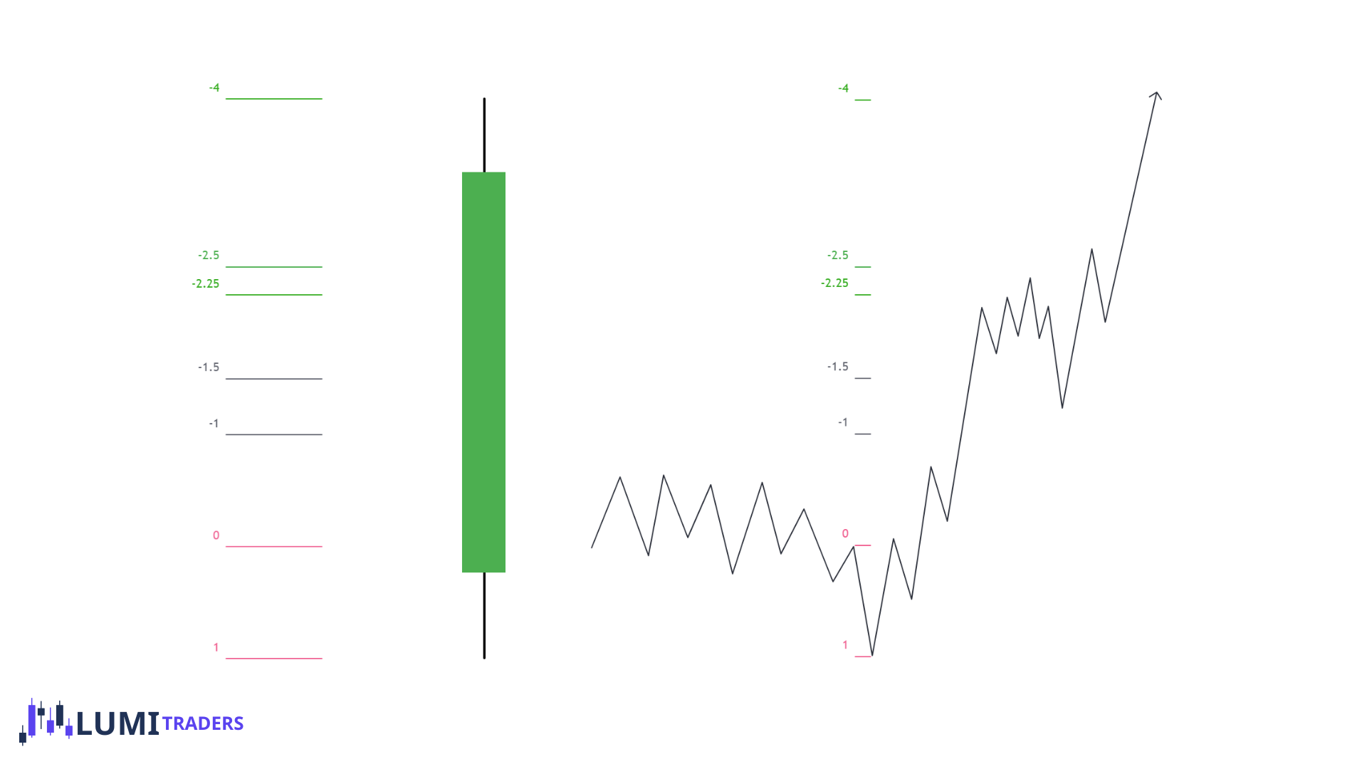
Manipulation phase usually occurs within the 2–2.5 Standard Deviation range of the consolidation leg projection.
How do I know when the Manipulation phase has finished?
Think in terms of MMXM. Always.
I look for the following elements:
1. HTF Level
2. LTF CISD
3. LTF Market Structure Shift (MSS)
4. SMT Divergence (optional)
Ideally, all of this occurs within the 2–2.5 STD range.
In order to confirm a transition from one program to another, we must have an HTF Level, LTF CISD, and LTF MSS. Only after these conditions are met can I draw the Manipulation Leg Projection.
I use the very last leg before the SMR, confirmed by both CISD and MSS, as my Manipulation Leg.
This final leg becomes the basis for my Manipulation Leg Projection, and ideally, the projected range should fall within the 2–2.5 Standard Deviation range.
Example
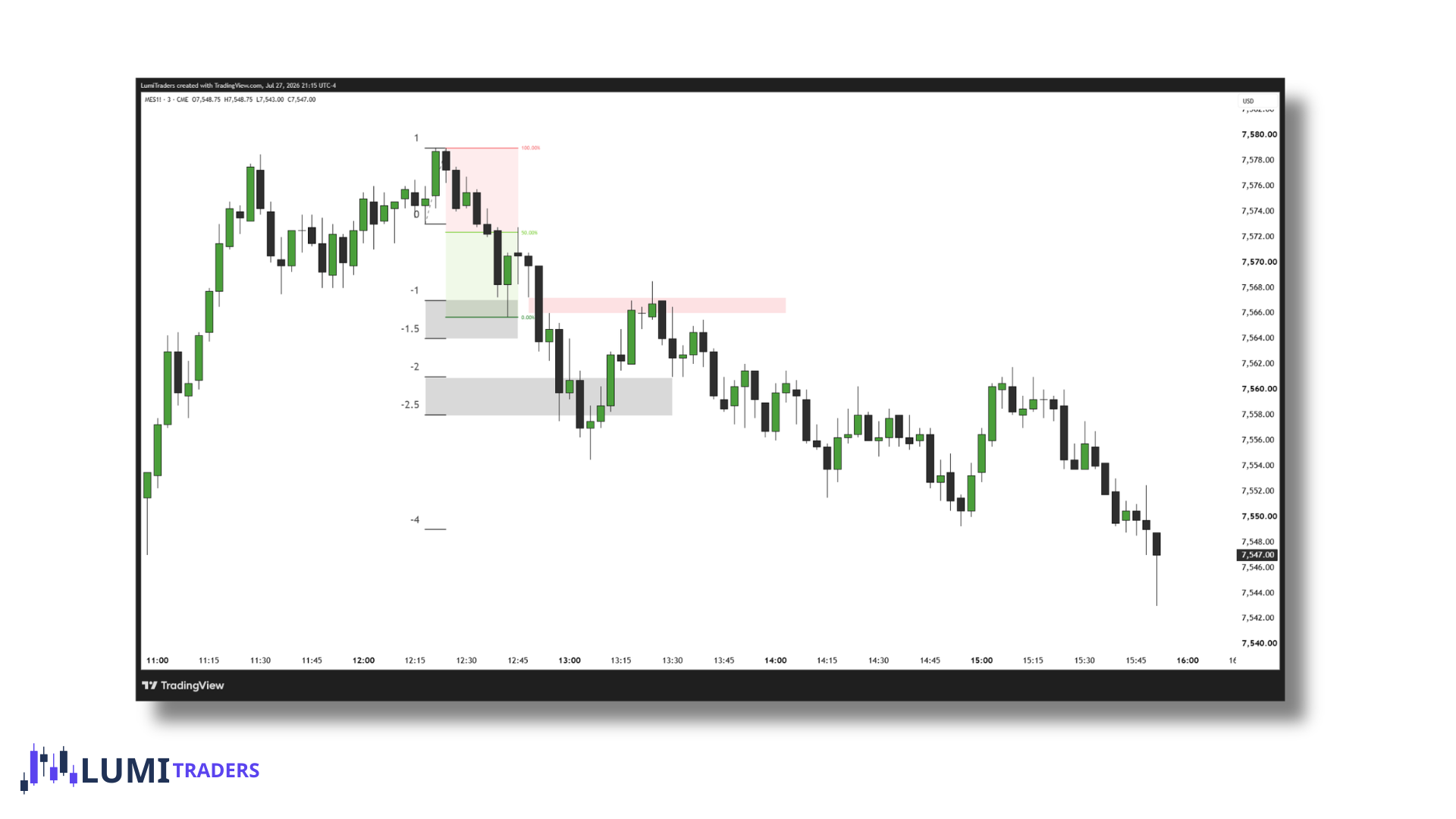
Standard Deviation Framework
I want to see SMR from a HTF PDA.
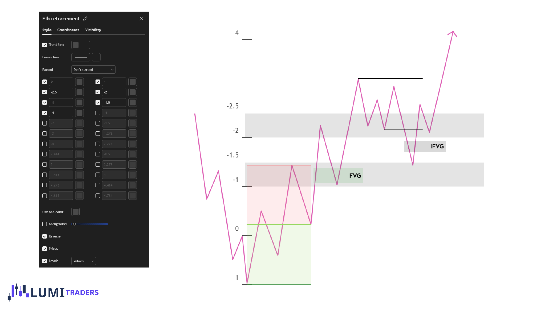
Once I have identified my Manipulation Leg, I will use the Fibonacci Retracement tool with the following levels:
1, 1.5, 2, and 4 Standard Deviations.
1–1.5 STDV: Retracement Range
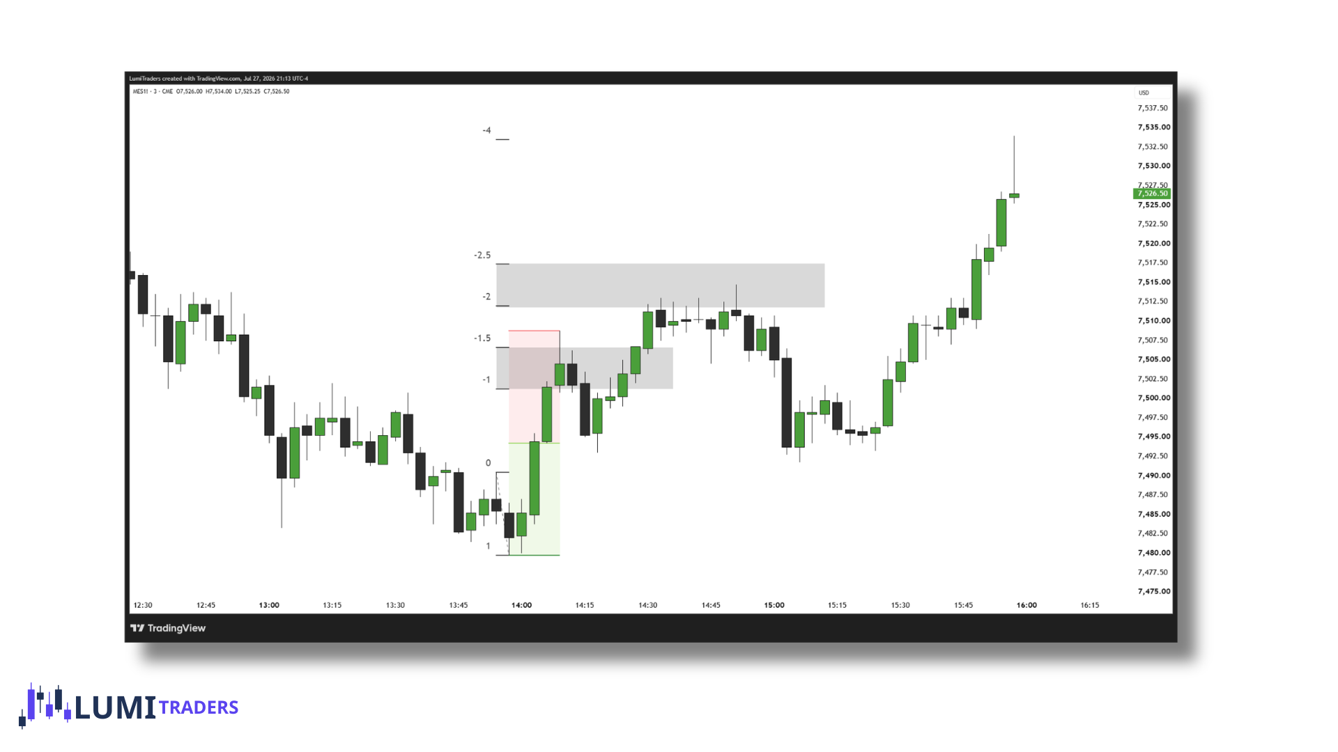
The range between 1 and 1.5 STDV will be my 1st Retracement Range.
Within this range, I am specifically interested in a retracement into the Equilibrium of the current dealing range. Price may trade into Premium or Discount, but more often, I expect Equilibrium to be respected.
Once price reaches the Equilibrium on the same timeframe used to measure the Manipulation Leg, I expect the move to continue toward the range between 2 and 2.5 STDV.
2–2.5 STDV: Last Retracement Range
This range will usually represent a part of the 2nd Stage of Re-Accumulation / Re-Distribution of MMXM.
Because of this, I expect to see Time Distortion (consolidation) develop within this range, which should provide the final setup needed to complete the MMXM.
Between 2 and 2.5 STDV, I want to see consolidation develop. Eventually, I expect price to run below the consolidation low or above the consolidation high.
Following this run, I will wait for an IFVG/CISD to form, which will provide my entry as part of the 2nd Stage of Re-Accumulation / Re-Distribution.
Ideally, after the Time Distortion high or low is raided, I want to see price deliver toward the FVG that formed within the 1–1.5 STDV range.
Impulse Leg
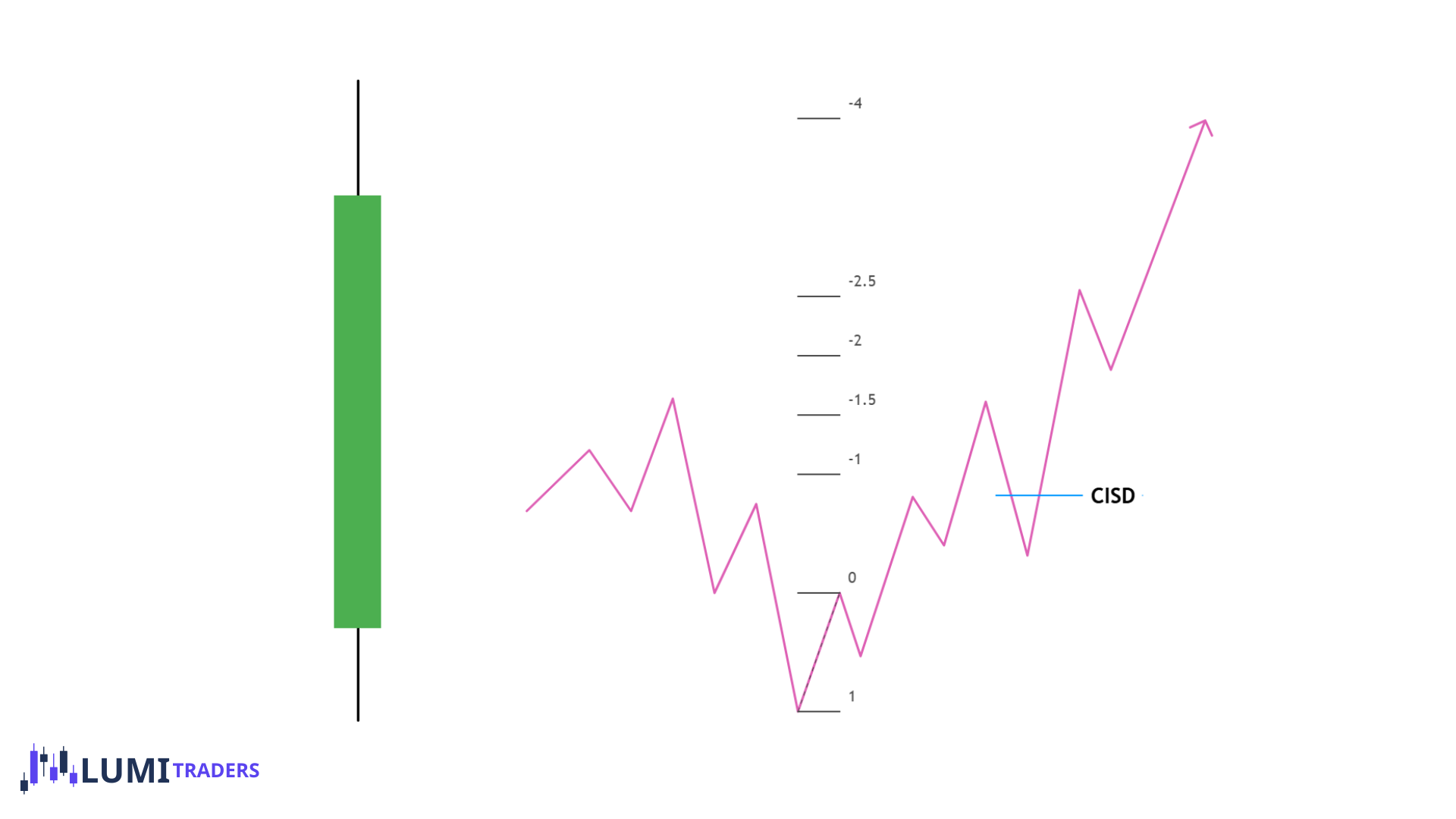
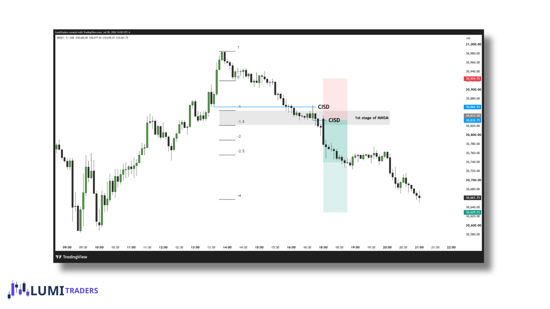
Impulse Leg Projection is a more conservative projection method that I use when the manipulation leg is unusually large.
I measure the very first impulsive move higher or lower after the SMR is confirmed. This move must occur before the first meaningful retracement. I then measure the impulse leg using the same approach that I use to measure the manipulation leg.
Unlike the manipulation leg projection, you usually will not see time distortion within the 2–2.5 standard deviation range. Most of the time, price will offer a move from the 1–1.5 standard deviation area instead. This is also where you may begin to see the first stage of accumulation or distribution forming.
Once again, I use this projection only when the manipulation leg is relatively large. Since I am not a swing trader, I use the impulse leg to identify a more conservative and realistic target that price can reach within the same trading day.
Time Distortion
What is Time Distortion
Time distortion is a period of price consolidation. As I mentioned earlier, it typically forms as part of the second stage of re-accumulation or re-distribution.
A common mistake is interpreting the initial move away from this consolidation as a Market Structure Shift and looking for a trade based on the 2022 Model.
However, instead of true continuation, price may make a false move below the time distortion low or above the time distortion high. It then reverses and continues delivering toward the higher-timeframe level to complete the MMXM.
This is why we should not treat every break of the time distortion range as a valid Market Structure Shift. We must wait for confirmation that the move is genuine rather than a liquidity sweep before the final delivery.
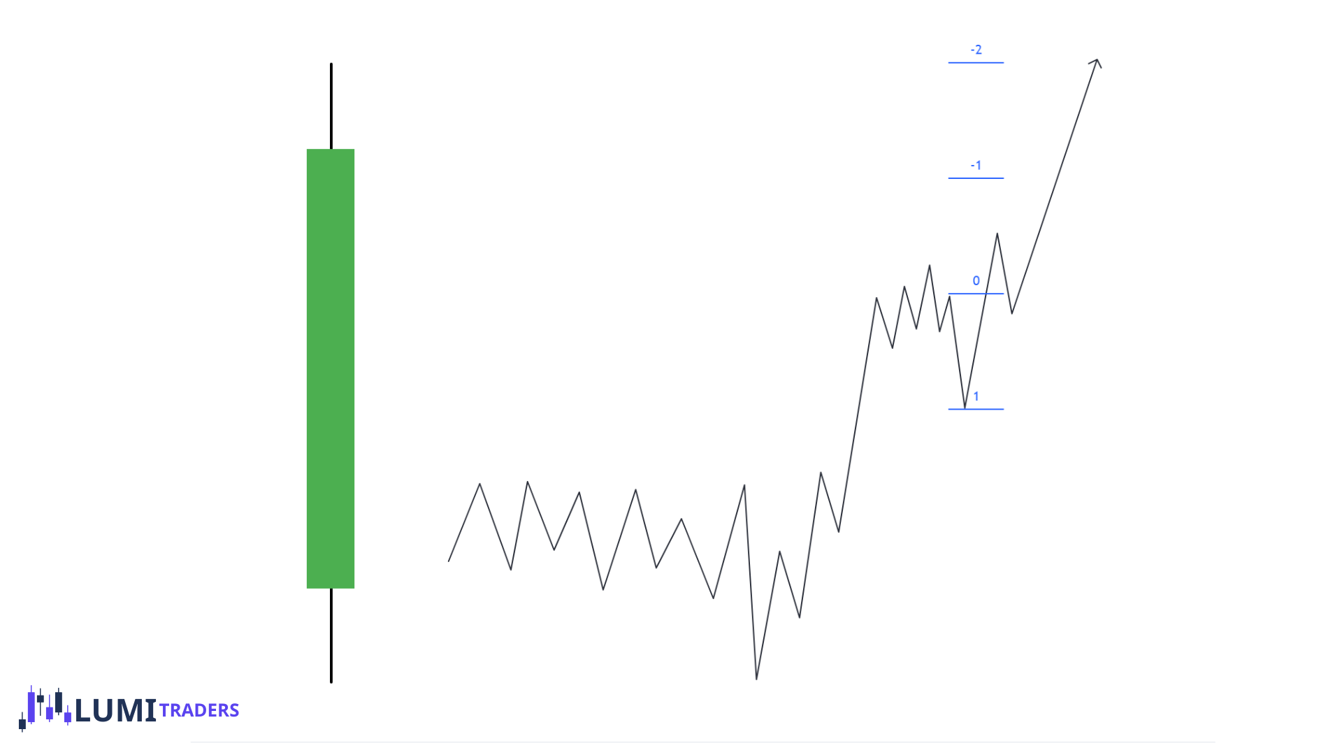
It is important to understand that during time distortion, market makers are accumulating long or short positions before completing the final move.
You will notice that price often begins to slow down near the 2–2.5 standard deviation range. This is exactly where we should avoid FOMO and resist the urge to chase the move.
Instead, understand that time—not price—will create the final opportunity.
We must remain patient and wait for price to break below or above the time distortion range before considering a trade. This breakout may initially appear to be a Market Structure Shift, but it often serves as the final liquidity manipulation before price reverses and completes the MMXM delivery.
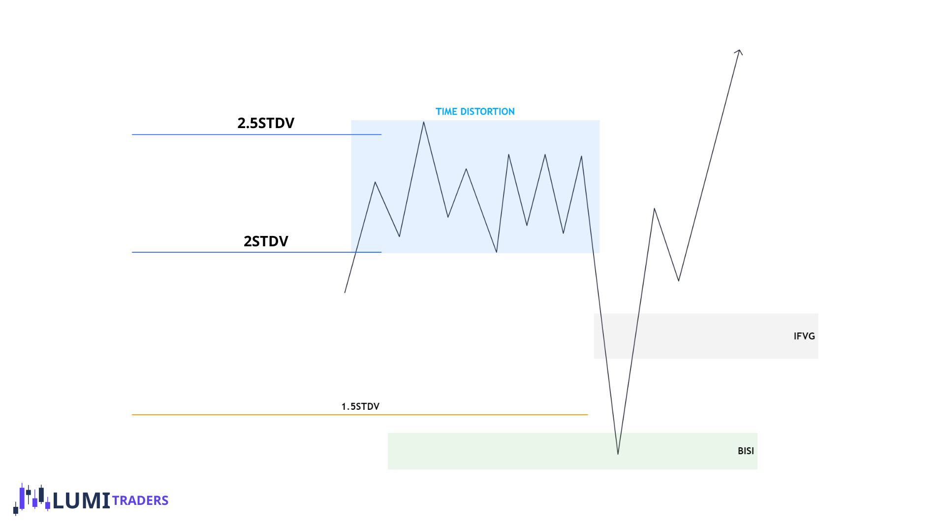
Now we understand that time distortion typically forms near the 2–2.5 standard deviation range of the manipulation leg projection.
If price remains below or above the higher-timeframe PDA, we can anticipate a retracement from the 2–2.5 standard deviation area. However, if price has already reached the higher-timeframe PDA, we should anticipate a potential reversal instead.
This retracement will often deliver price back into the 1–1.5 standard deviation range. Ideally, we want to see price reach a BISI or SIBI located within this area.
Once price breaks below the time distortion low or above the time distortion high, we can treat this move as another manipulation. This secondary manipulation is part of the second stage of re-accumulation or re-distribution.
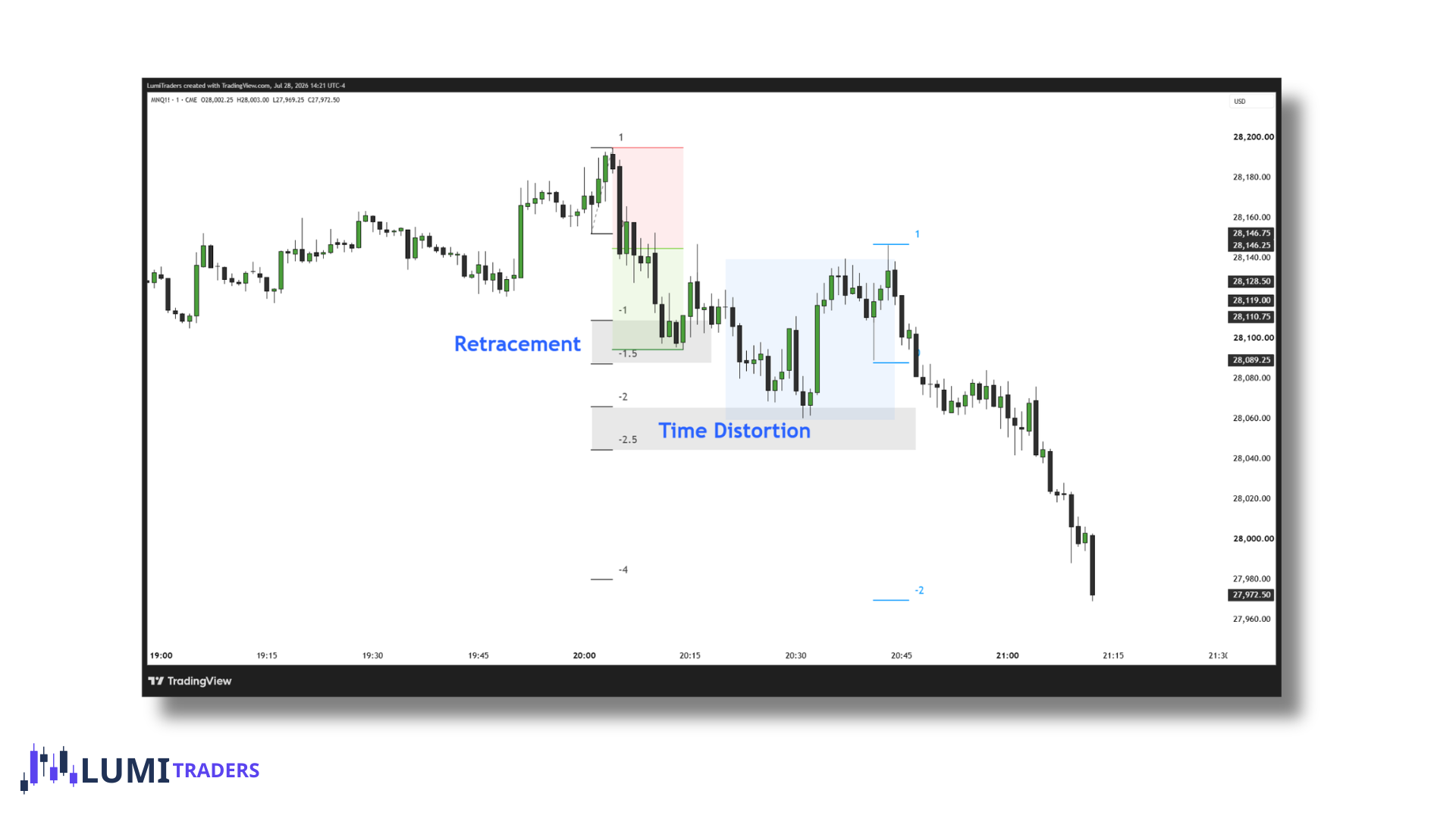
We then use the entire impulsive leg that broke the distortion low or high and project a 2-standard-deviation move from it.
Most of the time, this 2-standard-deviation projection will align with the 4-standard-deviation target of the original manipulation leg. I primarily use this alignment as additional confirmation for my take-profit level.
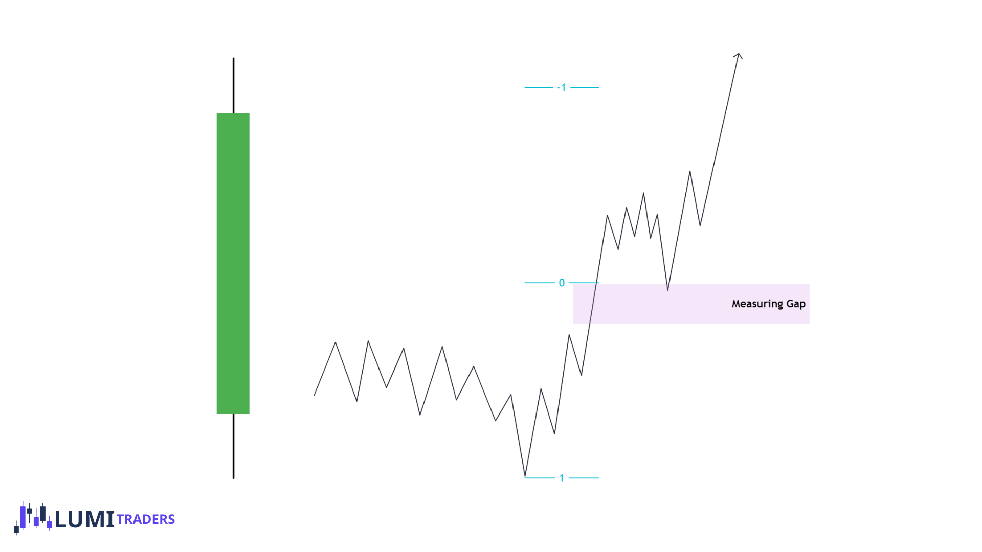
Measuring Gap
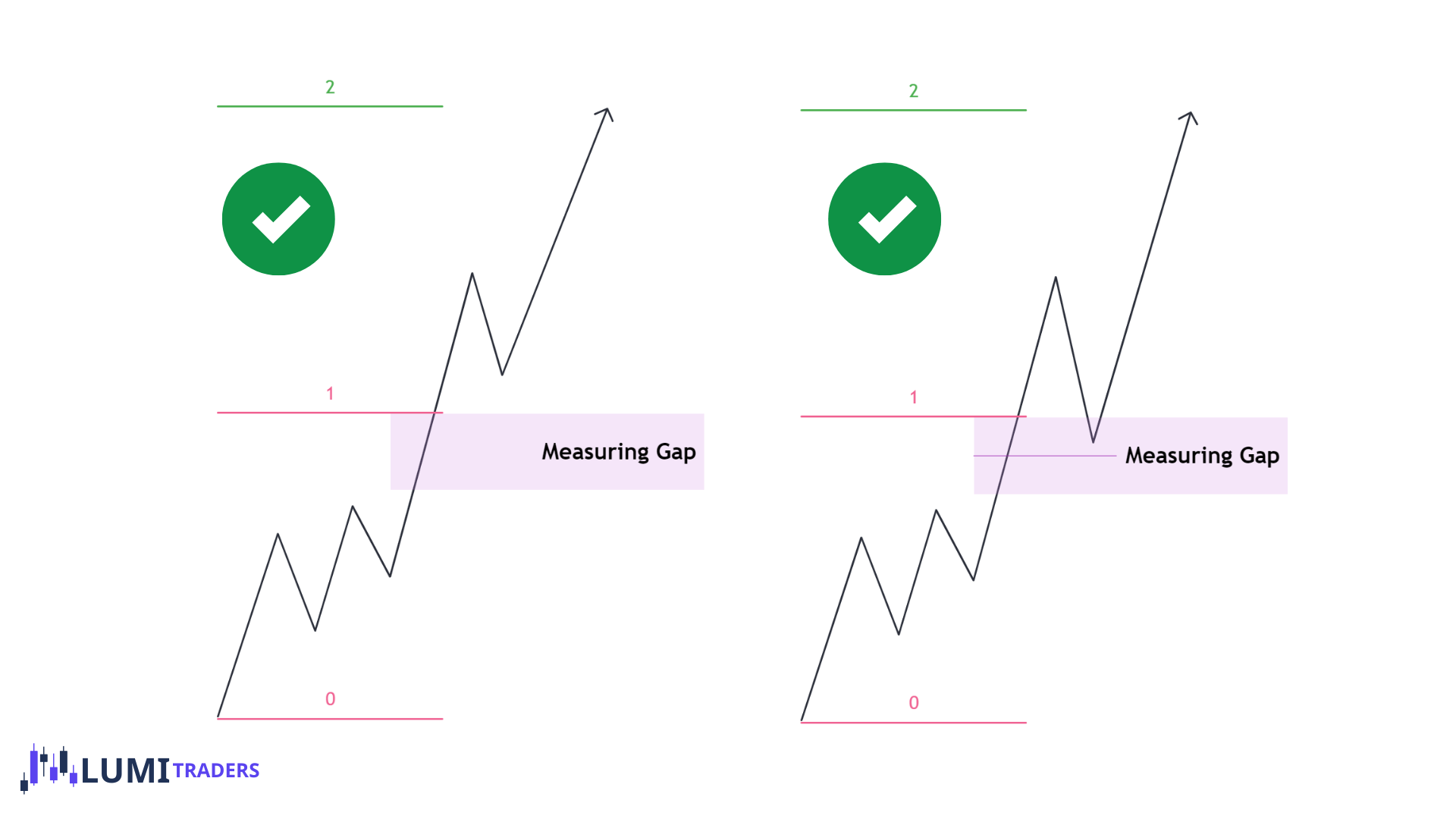
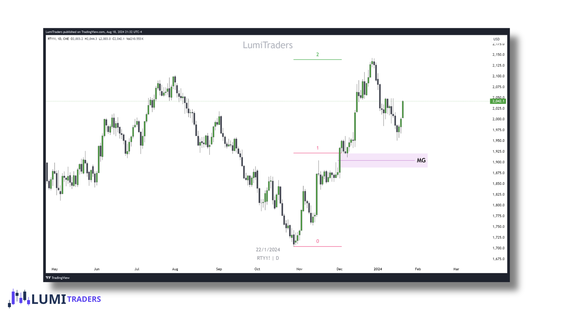
A Measuring Gap (MG) is a Fair Value Gap (FVG) that typically forms near the midpoint of an implied range. Unlike other types of gaps, a Measuring Gap often remains unfilled. When price does revisit it, the retracement is usually shallow, offering an IOFED (Institutional Order Flow Entry Drill) before continuing in the original direction to complete the formation of the implied range.
The Measuring Gap (MG) typically appears as a relatively large Fair Value Gap (FVG).
I generally use the projected move from the Measuring Gap as my MMXM target/terminus.
To reiterate, the Measuring Gap is the FVG located at the midpoint (50%) of the implied dealing range. /usually it forms during the second stage of re-accumulation or re-distribution.
To calculate the measuring move, I use:
The low/high where the SMR occurred, and
The top/bottom of the Measuring Gap.
Projecting this measurement by 100% provides my MMXM target.